Background

Perturbed spherical harmonic basis: temperature map

The photospheric temperature of an exoplanet, as a function of the planetary latitude \(\theta\) and longitude \(\phi\) can be defined as:

\[T = T_\mathrm{eq} (1 - A_B)^{1/4} \left( 1 + \sum_{m, \ell}^{\ell_{\rm max}} h_{m\ell}(\theta, \phi) \right)\]

such that \(T_\mathrm{eq} = f T_\mathrm{eff} \sqrt{R_\star/a}\) is the equilibrium temperature for greenhouse factor \(f\), stellar effective temperature \(T_\mathrm{eff}\), and normalized semimajor axis \(a/R_\star\); \(A_B\) is the Bond albedo. The prefactor on the left acts as a constant scaling term for the absolute temperature field, on which the \(h_{ml}\) terms are a perturbation.

The \(h_{m\ell}(\alpha, \omega_\mathrm{drag})\) terms are defined by:

\[\begin{split}\begin{split} h_{m\ell} = \frac{C_{m\ell}}{\omega_\mathrm{drag}^2 \alpha^4 + m^2} e^{-\tilde{\mu}/2} [ \mu m H_{\ell} \cos(m \phi) \\ + \alpha \omega_\mathrm{drag} (2lH_{\ell-1} - \tilde{\mu}H_\ell) \sin(m\phi) ], \end{split}\end{split}\]

where

\[\alpha = \mathcal{R}^{-1/2} \mathcal{P}^{-1/4}\]

is the dimensionless fluid number of Heng & Workman (2014), and is a function of the Reynold’s number \(\mathcal{R}\) and the Prandtl number \(\mathcal{P}\). \(\omega_\mathrm{drag}\) is the dimensionless drag frequency, \(\mu = \cos\theta\), \(\tilde{\mu}=\alpha \mu\), \(H_\ell(\tilde{\mu})\) are the Hermite polynomials:

\[\begin{split}\begin{eqnarray} H_0 &=& 1\\ H_1 &=& 2\tilde{\mu}\\ H_3 &=& 8\tilde{\mu}^3 - 12 \tilde{\mu}\\ H_4 &=& 16\tilde{\mu}^4 - 48\tilde{\mu}^2 + 12. \end{eqnarray}\end{split}\]

Phase curve

We can then compute the thermal flux emitted by the planet at any orbital phase \(\xi\), which is normalized from zero at secondary eclipse and \(\pm\pi\) at transit:

\[F_p = R_p^2 \int_{-\xi-\pi/2}^{-\xi+\pi/2} \int_0^\pi \mathcal{B}(T) \sin^2\theta \cos(\phi + \xi)d\theta d\phi\]

given the blackbody function defined as:

\[\mathcal{B}(T) = \int_{\lambda_1}^{\lambda_2} B_\lambda(T(\theta, \phi)) \mathcal{F}_\lambda d\lambda\]

where \(T(\theta, \phi)\) is the temperature map described with the perturbed spherical harmonic basis functions in the previous section, and \(\mathcal{F_\lambda}\) is the filter throughput.

The observation that we seek to fit is the infrared phase curve of the exoplanet, typically normalized as a ratio of the thermal flux of the planet normalized by the thermal flux of the star, like so:

\[F_p/F_\star = \frac{1}{\pi I_\star} \left(\frac{R_p}{R_\star}\right)^2 \int_0^\pi \int_{-\xi-\pi/2}^{-\xi+\pi/2} I_p(\theta, \phi) \cos(\phi+\xi) \sin^2(\theta) d\phi d\theta \label{eqn:diskint}\]

where the intensity \(I\) is given by

\[I = \int \mathcal{F}_\lambda \mathcal{B}_\lambda(T(\theta, \phi) d\lambda\]

for a filter bandpass transmittance function \(\mathcal{F}_\lambda\).

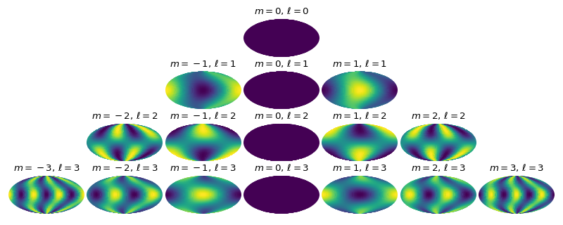
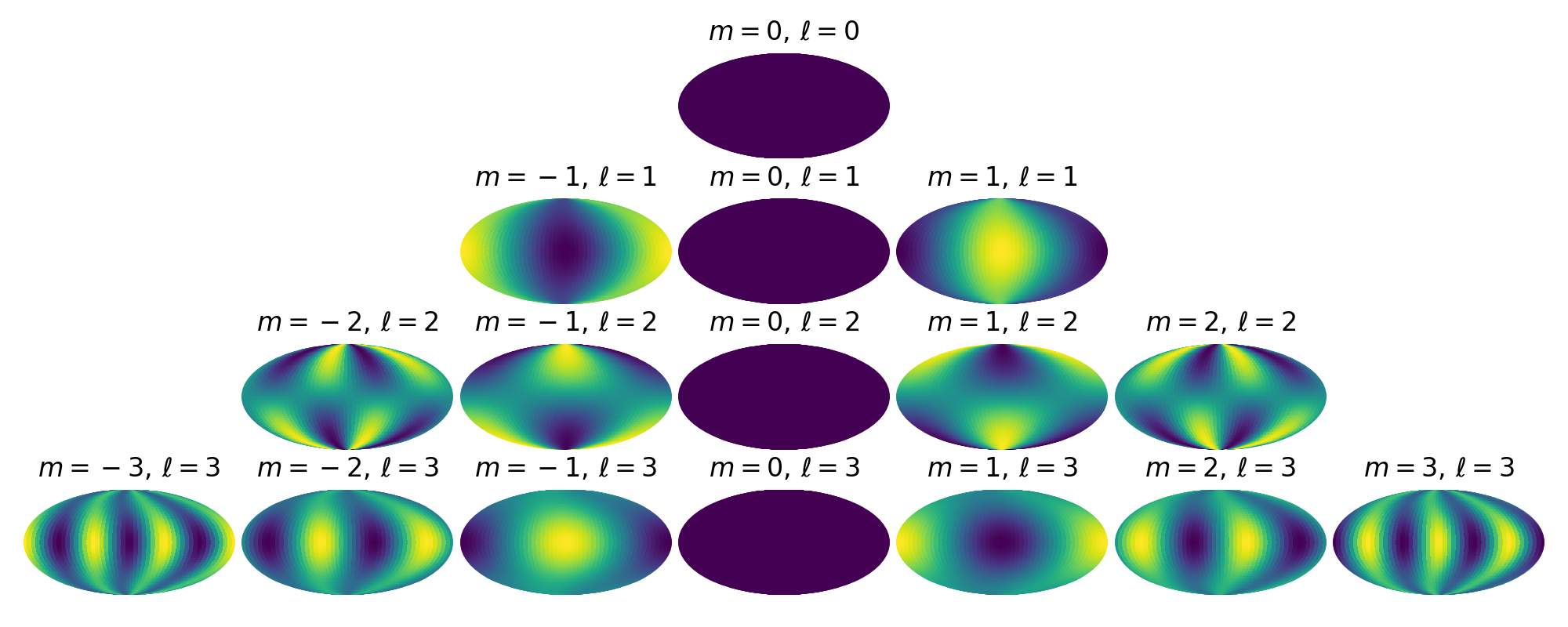
Example temperature fields

The first several terms in the spherical harmonic expansion of the temperature map in the \(h_{m\ell}\) basis. Each subplot shows the temperature perturbation (purple to yellow is cold to hot) as a function of latitude and longitude (shown in Mollweide projections such that the substellar longitude is in the center of the plot). The \(m = 0\) terms are always zero. The \(\ell=2\) terms are asymmetric about the equator and therefore do not represent typical GCM results, so we keep all \(\ell=2\) terms fixed to zero in the subsequent fits. These maps were generated with \(\alpha=0.6\) and \(\omega_\mathrm{drag} = 4.5\).

(Source code, png, hires.png, pdf)

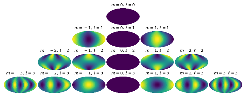
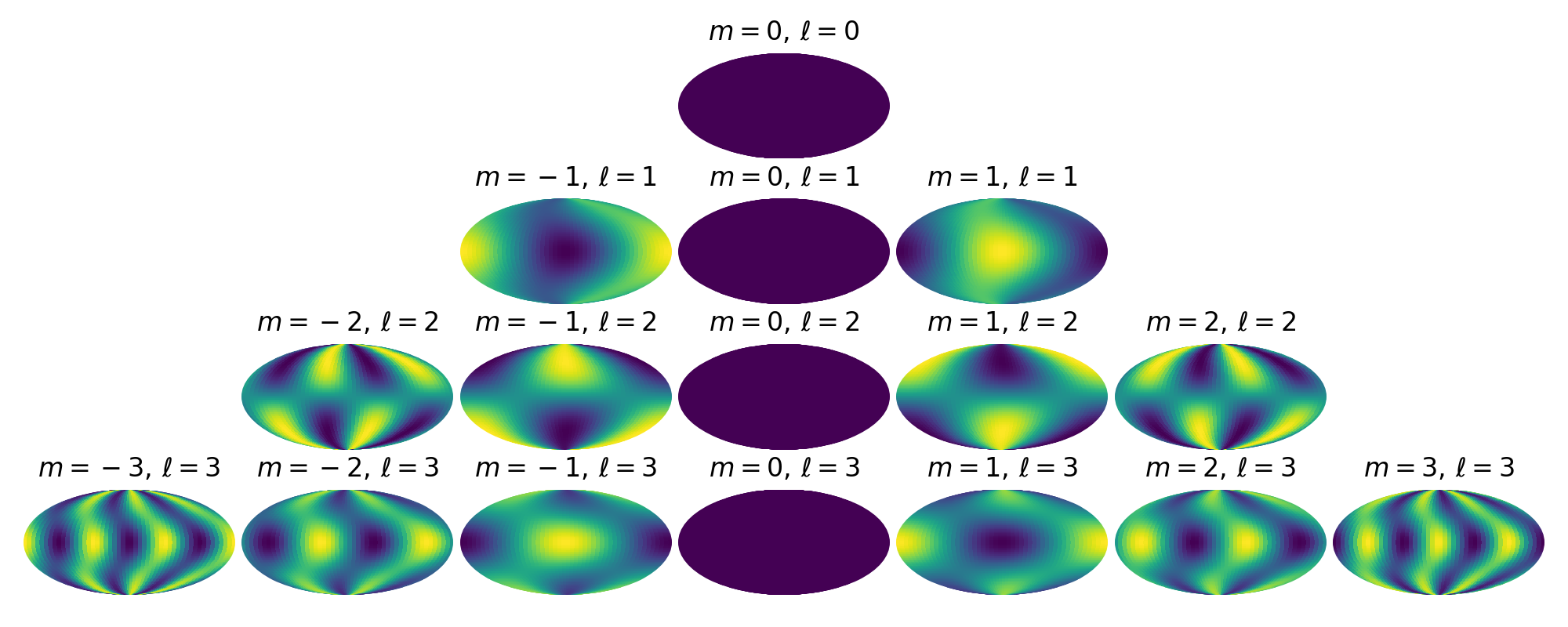
Below is the same as above, but this time for \(\alpha=0.9\) and \(\omega_\mathrm{drag} = 1.5\) – note that when the drag is set to a smaller value, the chevron shape becomes more pronounced as a perturbation on the temperature maps with \(\ell \neq 0\).

(Source code, png, hires.png, pdf)