Getting Started
Representing a planetary system with the \(h_{m\ell}\) basis
First, we’ll import the necessary packages:
import matplotlib.pyplot as plt
import numpy as np

from kelp import Filter, Planet, Model
Next we set some parameters for the model:
# Set phase curve parameters
hotspot_offset = -0.8  # hotspot offset [rad]
alpha = 0.6
omega_drag = 4.5
c11 = 0.18        # Spherical harmonic power C_{m=1, l=1}

# Set observation parameters
n = 'HD 189733'     # name of the planetary system
channel = 1         # Spitzer IRAC channel of observations
n_theta = 100        # number of latitudes to simulate
n_phi = 50          # number of longitudes to simulate
We initialize a Planet and Filter object for the model:
# Import planet properties
p = Planet.from_name(n)

# Import IRAC filter properties
filt = Filter.from_name(f"IRAC {channel}")
filt.bin_down(bins=10)  # this speeds up the example
We specify the \(C_{m\ell}\) terms like so:
# These elements will be accessed like C_ml[m][l]:
C_ml = [[0],
        [0, c11, 0]]
Let’s construct a Model object,
# Generate an h_ml basis model representation of the system:
model = Model(hotspot_offset=hotspot_offset,
              omega_drag=omega_drag,
              alpha=alpha, C_ml=C_ml, lmax=1, A_B=0,
              planet=p, filt=filt)
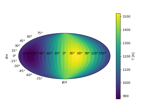
and plot the temperature map using temperature_map:
# Compute the temperature map:
T, theta, phi = model.temperature_map(n_theta, n_phi, f=2**-0.5)

# Plot the temperature map
fig = plt.figure()
ax = fig.add_subplot(111, projection='mollweide')
cax = ax.pcolormesh(phi, theta - np.pi/2, T)
plt.colorbar(cax, label='T [K]')
plt.show()
(Source code, png, hires.png, pdf)
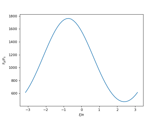
and plot the phase curve that results from this temperature map using
thermal_phase_curve:
# Compute the phase curve:
xi = np.linspace(-np.pi, np.pi, 50)
phase_curve = model.thermal_phase_curve(xi)

# Plot the phase curve
phase_curve.plot()
plt.xlabel('$\\xi/\\pi$')
plt.ylabel('$F_p/F_s$')
plt.show()
(Source code, png, hires.png, pdf)