Optimization
scipy and emcee
First let’s import the necessary packages, which include scipy and
emcee for non-linear optimization and MCMC respectively.
import matplotlib.pyplot as plt
import numpy as np

from kelp import Model, Planet, Filter

from scipy.optimize import minimize

from emcee import EnsembleSampler
from multiprocessing import Pool
from corner import corner

np.random.seed(42)
Next let’s set up the properties of the Planet, which we’ll assume is
like HD 189733 b, and the Filter which we’ll assume is the Spitzer/IRAC
Channel 1 (3.6 micron):
planet = Planet.from_name('HD 189733')
filt = Filter.from_name("IRAC 1")
filt.bin_down(10)  # this speeds up the integration
We’ll also set up the model parameters using the \(h_{m\ell}\) basis:
hotspot_offset = np.radians(-40)  # Hotspot offset
alpha = 0.6          # dimensionless fluid number
omega = 4.5          # dimensionless drag frequency
f = 2**-0.5          # greenhouse parameter
A_B = 0              # Bond albedo
lmax = 1             # \ell_{max}
C = [[0],            # C_{m \ell} terms
     [0, 0.15, 0]]
obs_err = 50         # Observational white noise
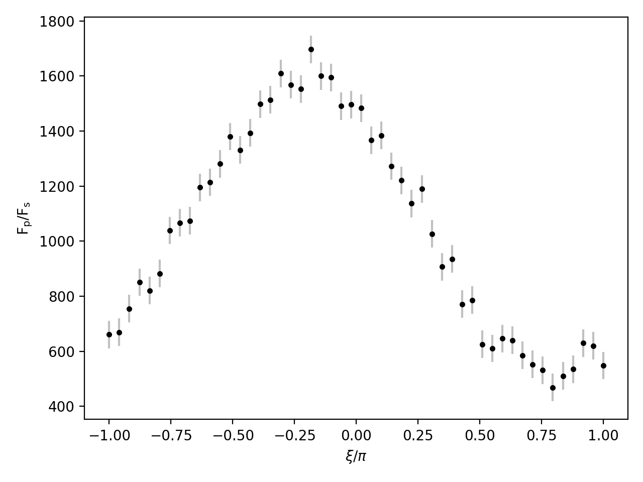
Now we’ll initialize a noisy instance of the model to be our “truth” in this example, which we will recover with optimization techniques:
# `xi` is the time axis of the phase curve, going from -pi (transit) to
# 0 (eclipse) and back to pi (transit)
xi = np.linspace(-np.pi, np.pi, 50)

# Compute the phase curve of the exoplanet:
model = Model(hotspot_offset, alpha, omega,
              A_B, C, lmax, planet=planet, filt=filt)
obs = model.thermal_phase_curve(xi, f=f).flux

# Add random noise to the light curve:
obs += obs_err * np.random.randn(xi.shape[0])

# Plot the simulated "observations"
errkwargs = dict(color='k', fmt='.', ecolor='silver')
plt.errorbar(xi / np.pi, obs, obs_err, **errkwargs)
plt.xlabel('$\\xi/\\pi$')
plt.ylabel('$\\rm F_p/F_s$')
(Source code, png, hires.png, pdf)
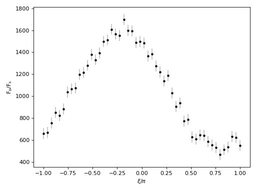
The simulated observations obs have small scale, uncorrelated scatter
about the phase curve mean model. Next we’ll use scipy to find the best-fit
values for the hotspot offset \(\Delta \phi\) and the power in the
\(C_{11}\) spherical harmonic coefficient term:
def pc_model(p, x):
    """
    Phase curve model with two free parameters
    """
    offset, c_11, f = p
    C = [[0],
         [0, c_11, 0]]
    model = Model(hotspot_offset=offset, alpha=alpha,
                  omega_drag=omega, A_B=A_B, C_ml=C, lmax=1,
                  planet=planet, filt=filt)
    return model.thermal_phase_curve(x, f=f, check_sorted=False).flux

def lnprior(p):
    """
    Log-prior: sets reasonable bounds on the fitting parameters
    """
    offset, c_11, f = p

    if (offset > np.pi or offset < -np.pi or c_11 > 1 or c_11 < 0):
        return -np.inf

    return 0

def lnlike(p, x, y, yerr):
    """
    Log-likelihood: via the chi^2
    """
    return -0.5 * np.sum((pc_model(p, x) - y)**2 / yerr**2)

def lnprob(p, x, y, yerr):
    """
    Log probability: sum of lnlike and lnprior
    """
    lp = lnprior(p)

    if np.isfinite(lp):
        return lp + lnlike(p, x, y, yerr)
    return -np.inf


initp = np.array([-0.7, 0.1])

bounds = [[0, 2], [0.1, 1]]

soln = minimize(lambda *args: -lnprob(*args),
                initp, args=(xi, obs, obs_err),
                method='powell')
soln.x now contains the best-fit (\(\Delta \phi\), \(C_{11}\))
parameters from Powell’s method. With this guess at the maximum a posteriori
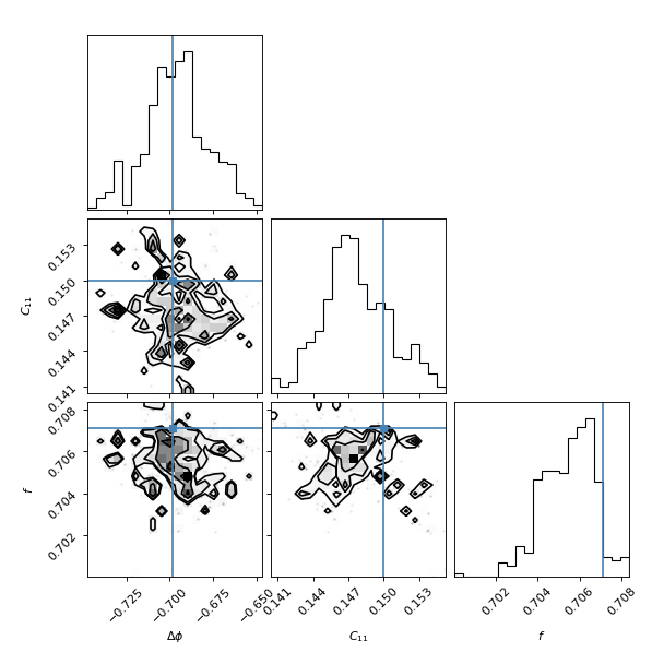
values for the free parameters, let’s now use Markov Chain Monte Carlo to
measure the uncertainty on the maximum-likelihood parameters:
ndim = 3
nwalkers = 2 * ndim # in real life, you should scale this factor up
# Generate initial positions for the walkers
p0 = [soln.x + 0.1 * np.random.randn(ndim)
for i in range(nwalkers)]
# Run the ensemble sampler:
with Pool() as pool:
sampler = EnsembleSampler(nwalkers, ndim, lnprob,
args=(xi, obs, obs_err),
pool=pool)
p1 = sampler.run_mcmc(p0, 100)
sampler.reset()
sampler.run_mcmc(p1, 500, progress=True)
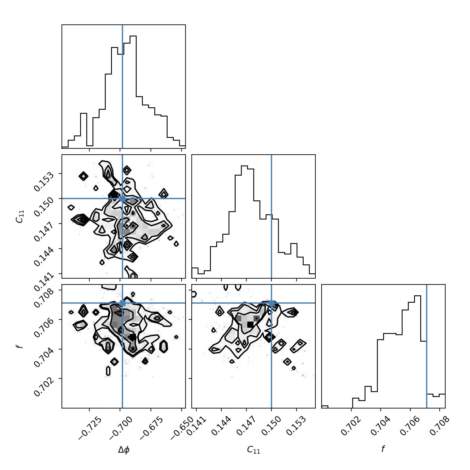
# Plot the corner plot with the posteriors:
corner(sampler.flatchain, truths=[hotspot_offset, C[1][1], 2**-0.5],
labels=['$\Delta \phi$', '$C_{11}$', '$f$'])
plt.show()
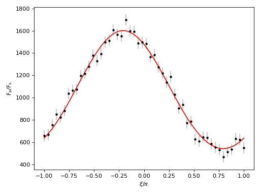
# Extract the maximum a posteriori parameters, plot the corresponding model
p_map = sampler.flatchain[np.argmax(sampler.flatlnprobability)]
plt.errorbar(xi/np.pi, obs, obs_err, **errkwargs)
plt.plot(xi/np.pi, pc_model(p_map, xi), color='r')
plt.xlabel('$\\xi/\\pi$')
plt.ylabel('$\\rm F_p/F_s$')
plt.show()
(Source code, png, hires.png, pdf)


The blue lines on the corner plot represent the “true” (input) values which we used to construct the simulated observations. The recovered (\(\Delta \phi\), \(C_{11}\)) parameters are consistent with their true values. The maximum likelihood parameters generate a model (red) that looks very consistent with the observations (black).
When doing this integration for non-demonstration purposes, you should tweak the number of walkers to be more like a factor of 5-10 greater than the number of dimensions, and the number of steps should be increased by a factor of at least a few.
PyMC3
The \(h_{m\ell}\) basis has also been implemented within kelp using theano for compatibility with PyMC3. Here’s a simple example that shows inference with the theano module:
import multiprocessing as mp
import numpy as np
import matplotlib.pyplot as plt
import astropy.units as u

import pymc3 as pm
from corner import corner

floatX = 'float32'

from kelp import theano, Model, Filter, Planet

np.random.seed(42)

planet = Planet.from_name('HD 189733')
filt = Filter.from_name("IRAC 1")
filt.bin_down(5)

# Set orbital phase axis:
xi = np.linspace(-np.pi, np.pi, 100)

hotspot_offset = np.radians(-40)
alpha = 0.6
omega = 4.5
true_f = 2 ** -0.5
A_B = 0
lmax = 1
true_C_11 = 0.15
C = [[0],
     [0, true_C_11, 0]]
obs_err = 50
model = Model(hotspot_offset, alpha, omega,
              A_B, C, lmax, planet=planet, filt=filt)
obs = model.thermal_phase_curve(xi, f=true_f).flux
obs += obs_err * np.random.randn(xi.shape[0])


# Set planet parameters:
lmax = 1
T_s = planet.T_s
a_rs = planet.a
rp_a = planet.rp_a

# Set resolution of grid points on sphere:
n_phi = 100
n_theta = 10
phi = np.linspace(-2 * np.pi, 2 * np.pi, n_phi, dtype=floatX)
theta = np.linspace(0, np.pi, n_theta, dtype=floatX)
theta2d, phi2d = np.meshgrid(theta, phi)

with pm.Model() as hml_model:
    delta_phi = pm.Uniform(
        "delta_phi", lower=np.radians(-90), upper=np.radians(90),
        testval=np.radians(-40)
    )
    C_11 = pm.Uniform(
        "C_11", lower=0.01, upper=0.3, testval=0.15
    )
    f = pm.Normal(
        "f", mu=2**-0.5, sigma=0.1
    )

    thermal_phase_curve, temperature_map, ps = theano.thermal_phase_curve(
        xi.astype(floatX), delta_phi,
        omega, alpha, C_11, T_s, a_rs, rp_a, A_B,
        theta2d.astype(floatX), phi2d.astype(floatX),
        filt.wavelength.to(u.m).value.astype(floatX),
        filt.transmittance.astype(floatX), true_f
    )

    pm.Normal(
        "obs", mu=thermal_phase_curve, observed=obs, sigma=obs_err
    )

    trace = pm.sample(
        draws=1000, tune=1000,
        compute_convergence_checks=False,
        mp_ctx=mp.get_context('fork')
    )

truths = {
    "delta_phi": hotspot_offset,
    "C_11": true_C_11,
    "f": true_f
}

df = pm.trace_to_dataframe(trace)[truths.keys()]
corner(
    df,
    truths=[truths[k] for k in truths.keys()]
)
plt.show()