Reflected Light

kelp implements the reflected light phase curve parameterization for an homogeneous planetary atmospheres as derived by Heng, Morris & Kitzmann (HMK; 2021). The HMK reflected light model is a function of two fundamental parameters which describe the scattering in the planetary atmosphere: the single-scattering albedo \(\omega\); and the scattering asymmetry factor \(g\).

Below, we’ll show how to use the reflected light formulation for a homogeneous planetary atmosphere to fit the Kepler phase curve of HAT-P-7 b; then we’ll move on to the case of an inhomogeneous atmosphere with the phase curve of Kepler-7 b.

Homogeneous reflectivity map

We can implement a model for the Kepler phase curve of HAT-P-7 b, which combines all aspects of a challenging phase curve (except atmospheric inhomogeneity, for this see the next section). HAT-P-7 b is a 2700 K planet with strong ellipsoidal variations, nearly-equal contributions to the Kepler phase curve from thermal emission and reflected light, plus detectable Doppler beaming. We’ll implement each of these contributions in the example below, and solve for the maximum-likelihood single-scattering albedo and scattering asymmetry factor, as well as the amplitudes of the Doppler beaming and ellipsoidal variations.

First we’ll import the necessary packages (there are quite a few!):

import numpy as np
import matplotlib.pyplot as plt
from scipy.stats import binned_statistic

import arviz
from corner import corner
import numpyro

# Set the number of cores on your machine for parallelism:
cpu_cores = 1
numpyro.set_host_device_count(cpu_cores)

from numpyro.infer import MCMC, NUTS
from numpyro import distributions as dist

from jax import numpy as jnp
from jax.random import PRNGKey, split

from lightkurve import search_lightcurve
from batman import TransitModel

import astropy.units as u
from astropy.constants import R_sun, R_earth
from astropy.stats import sigma_clip, mad_std

from kelp import Filter, Planet
from kelp.jax import reflected_phase_curve, thermal_phase_curve

Note that we have imported the phase curve functions from the jax module, because we will be using numpyro to construct the model and draw posterior samples.

Now we will define the system parameters that we will use to construct the phase curve and phase fold the light curve:

b = 0.4960  # Esteves 2015
r_star = 1.991 * R_sun
a_rs = 4.13 # Stassun 2017
inc = np.degrees(np.arccos(b / a_rs))
period = 2.204740  # Stassun 2017
t0 = 2454954.357462  # Bonomo 2017
rp_rs = float(16.9 * R_earth / r_star)  # Stassun 2017, Berger 2017
a_rp = float(a_rs / rp_rs)
T_s = 6449  # Berger 2018

p = Planet(
    per=period,
    t0=t0,
    rp=rp_rs,
    a=a_rs,
    inc=inc,
    u=[0.0, 0.0],
    fp=1.0,
    t_secondary=t0 + period/2,
    T_s=T_s,
    rp_a=1/a_rp,
    w=90,
    ecc=0,
    name="HAT-P-7"
)
p.duration = 4.0398 / 24  # Holczer 2016
rho_star = 0.27 * u.g / u.cm ** 3  # Stassun 2017
eclipse_half_dur = p.duration / p.per / 2

Now we will use search_lightcurve to download the long cadence light curve from Quarter 10 of the Kepler observations of HAT-P-7 b. We’ll then “flatten” the light curve, which applies a savgol filter to the light curve to do some long-term detrending on the out-of-transit portions of the phase curve. We will also sigma-clip the fluxes to remove outliers:

lcf = search_lightcurve(
    p.name, mission="Kepler", cadence="long", quarter=10, author="Kepler"
).download_all()

slc = lcf.stitch()

phases = ((slc.time.jd - t0) % period) / period
in_eclipse = np.abs(phases - 0.5) < eclipse_half_dur
in_transit = (phases < 1.5 * eclipse_half_dur) | (
        phases > 1 - 1.5 * eclipse_half_dur)
out_of_transit = np.logical_not(in_transit)

slc = slc.flatten(
    polyorder=3, break_tolerance=10,
    window_length=1001, mask=~out_of_transit
).remove_nans()

phases = ((slc.time.jd - t0) % period) / period
in_eclipse = np.abs(phases - 0.5) < eclipse_half_dur
in_transit = (phases < 1.5 * eclipse_half_dur) | (
        phases > 1 - 1.5 * eclipse_half_dur)
out_of_transit = np.logical_not(in_transit)

sc = sigma_clip(
    slc.flux[out_of_transit],
    maxiters=100, sigma=8, stdfunc=mad_std
)

Next we will compute the masked phases, times, and the normalized fluxes \(F_p/F_\mathrm{star}\) in units of ppm:

phase = phases[out_of_transit][~sc.mask]
time = slc.time.jd[out_of_transit][~sc.mask]

bin_in_eclipse = np.abs(phase - 0.5) < eclipse_half_dur
unbinned_flux_mean = np.mean(sc[~sc.mask].data)

unbinned_flux_mean_ppm = 1e6 * (unbinned_flux_mean - 1)
flux_normed = (
    1e6 * (sc[~sc.mask].data / unbinned_flux_mean - 1.0)
)
flux_normed_err = (
    1e6 * slc.flux_err[out_of_transit][~sc.mask].value
)

Now we will median-bin the phase folded Kepler light curve:

bins = 250
bs = binned_statistic(
    phase, flux_normed, statistic=np.median, bins=bins
)

bs_err = binned_statistic(
    phase, flux_normed_err,
    statistic=lambda x: 3 * np.median(x) / len(x) ** 0.5, bins=bins
)

binphase = 0.5 * (bs.bin_edges[1:] + bs.bin_edges[:-1])
# Normalize the binned fluxes by the in-eclipse flux:
binflux = bs.statistic - np.median(bs.statistic[np.abs(binphase - 0.5) < 0.01])
binerror = bs_err.statistic

Now we will use the Filter object to define the filter transmittance curve for Kepler:

filt = Filter.from_name("Kepler")
filt.bin_down(6)   # This speeds up integration by orders of magnitude
filt_wavelength, filt_trans = filt.wavelength.to(u.m).value, filt.transmittance

We compute the eclipse model once, it will not vary in the MCMC:

# Compute the eclipse model (no limb-darkening),
# normalize the eclipse model to unity out of eclipse and
# zero in-eclipse
eclipse = TransitModel(
    p, binphase * period + t0,
    transittype='secondary',
).light_curve(p) - 1

Next we construct the numpyro model. This is a long block of code, so let’s jump straight into in-line comments:

def model():
    # Define reflected light phase curve model according to
    # Heng, Morris & Kitzmann (2021)
    omega = numpyro.sample(
        'omega', dist.Uniform(low=0, high=1)
    )
    g = numpyro.sample('g',
        dist.TwoSidedTruncatedDistribution(
            dist.Normal(loc=0, scale=0.4),
            low=0, high=1
        )
    )
    reflected_ppm, A_g, q = reflected_phase_curve(binphase, omega, g, a_rp)

    # Define the ellipsoidal variation parameterization (simple sinusoid)
    ellipsoidal_amp = numpyro.sample(
        'ellip_amp', dist.Uniform(
            low=0, high=50
        )
    )
    ellipsoidal_model_ppm = - ellipsoidal_amp * jnp.cos(
        4 * np.pi * (binphase - 0.5)
    ) + ellipsoidal_amp

    # Define the doppler variation parameterization (simple sinusoid)
    doppler_amp = numpyro.sample(
        'doppler_amp', dist.Uniform(low=0, high=50)
    )
    doppler_model_ppm = doppler_amp * jnp.sin(
        2 * np.pi * binphase
    )

    # Define the thermal emission model according to description in
    # Morris et al. (in prep)
    xi = 2 * np.pi * (binphase - 0.5)
    n_phi = 75
    n_theta = 5
    phi = np.linspace(-2 * np.pi, 2 * np.pi, n_phi)
    theta = np.linspace(0, np.pi, n_theta)
    theta2d, phi2d = np.meshgrid(theta, phi)

    ln_C_11_kepler = -2.6
    C_11_kepler = jnp.exp(ln_C_11_kepler)
    hml_eps = 0.72
    hml_f = (2 / 3 - hml_eps * 5 / 12) ** 0.25
    delta_phi = 0

    A_B = 0.0

    # Compute the thermal phase curve with zero phase offset
    thermal, T = thermal_phase_curve(
        xi, delta_phi, 4.5, 0.575, C_11_kepler, T_s, a_rs, 1 / a_rp, A_B,
        theta2d, phi2d, filt_wavelength, filt_trans, hml_f
    )

    # Define the composite phase curve model
    flux_norm = eclipse * (
        reflected_ppm + ellipsoidal_model_ppm +
        doppler_model_ppm + 1e6 * thermal
    )

    # Keep track of the geometric albedo and integral phase function at
    # each step in the chain
    numpyro.deterministic('A_g', A_g)
    numpyro.deterministic('q', q)
    numpyro.deterministic('light_curve', flux_norm)

    # Define the likelihood
    numpyro.sample(
        "obs", dist.Normal(
            loc=flux_norm,
            scale=binerror
        ), obs=binflux
    )

Now our model is set up, and we are ready to draw posterior samples from the model given the data, which we will do with numpyro for the most efficient posterior sampling of our degenerate phase curve parameterization. This will take a few seconds:

# Random numbers in jax are generated like this:
rng_seed = 42
rng_keys = split(
    PRNGKey(rng_seed),
    cpu_cores
)

# Define a sampler, using here the No U-Turn Sampler (NUTS)
# with a dense mass matrix:
sampler = NUTS(
    model,
    dense_mass=True
)

# Monte Carlo sampling for a number of steps and parallel chains:
mcmc = MCMC(
    sampler,
    num_warmup=500,
    num_samples=2_000,
    num_chains=cpu_cores
)

# Run the MCMC
mcmc.run(rng_keys)

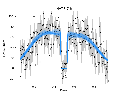
Let’s finally plot the final results:

# arviz converts a numpyro MCMC object to an `InferenceData` object based on xarray:
result = arviz.from_numpyro(mcmc)

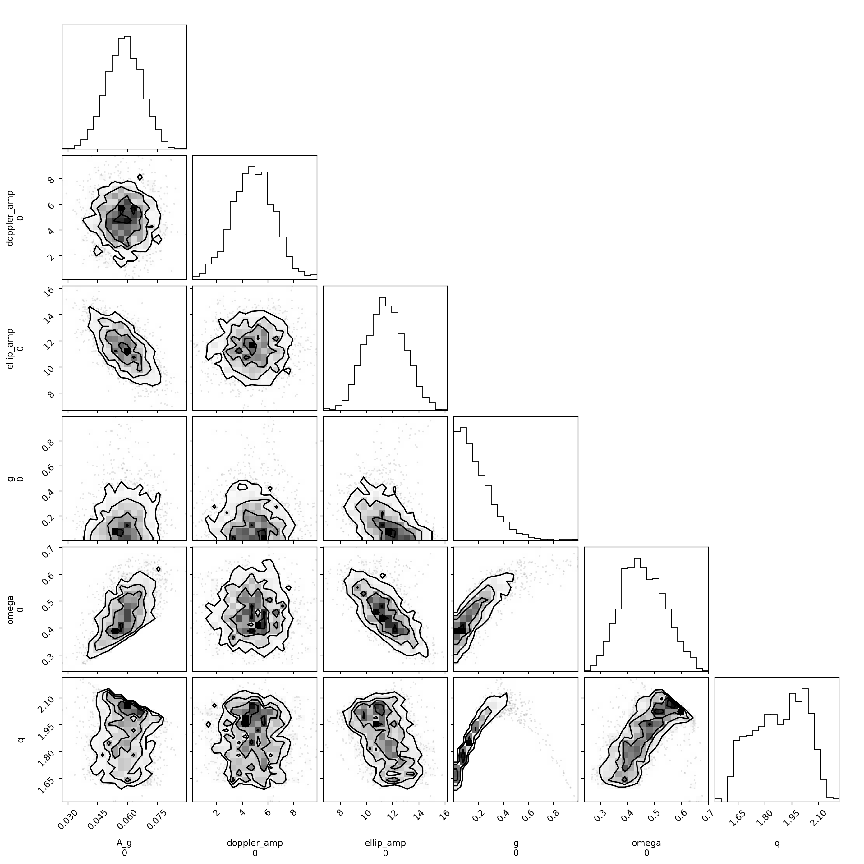
corner(result, var_names=["~light_curve"])
plt.show()

plt.figure()
plt.errorbar(
    binphase, binflux, binerror,
    fmt='.', color='k', ecolor='silver'
)

# plot a few samples of the model
random_indices = np.random.randint(
    0, mcmc.num_samples, size=50
)
for i in random_indices:
    plt.plot(
        binphase,
        np.array(result.posterior['light_curve'][0, i]),
        color='DodgerBlue', alpha=0.2, zorder=10
    )

plt.ylim([-30, 110])
for sp in ['right', 'top']:
    plt.gca().spines[sp].set_visible(False)
plt.gca().set(xlabel='Phase', ylabel='$F_p/F_\mathrm{star}$ [ppm]',
              title='HAT-P-7 b')
plt.show()

(Source code, png, hires.png, pdf)

(png, hires.png, pdf)

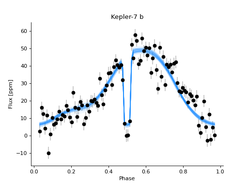
In the above corner plot, you’ll see the joint posterior correlation plots for each of the free parameters in the fit, including the single-scattering albedo \(\omega\), the scattering asymmetry factor \(g\), and the derived parameters including the Bond albedo \(A_B\), the geometric albedo \(A_g\), and the integral phase function \(q\).

You’ll also see a plot above with several draws from the posteriors for each parameter plotted in light-curve space, showing the range of plausible contributions from each phase curve component shown in different colors.

Inhomogeneous reflectivity map

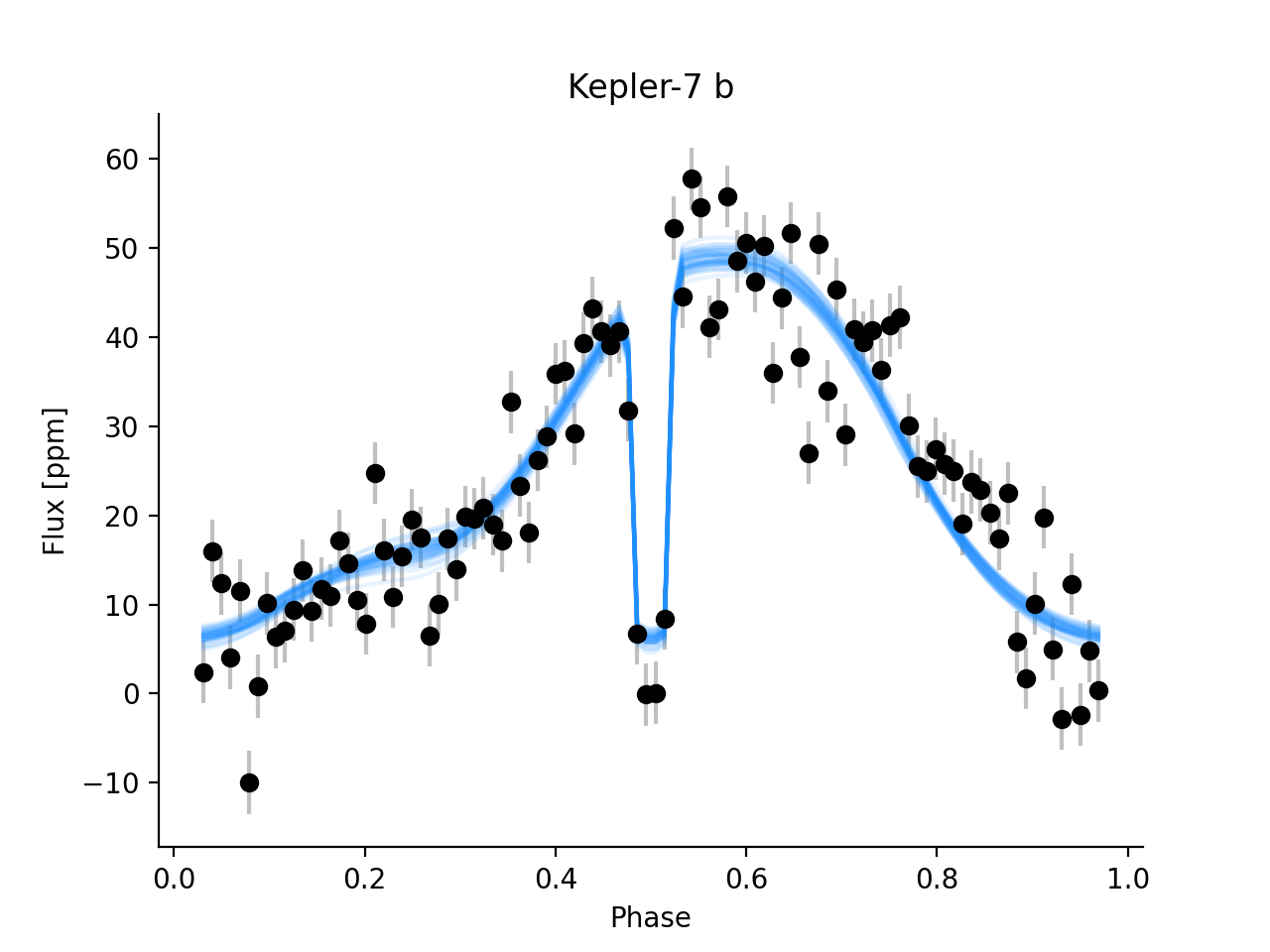
Kepler-7 b is a warm Jupiter with an insignificant thermal emission contribution to the Kepler phase curve, but with a significant phase curve asymmetry, possibly resulting from an inhomogeneous albedo distribution on the surface of the planet. In this example, we’ll give two parameters for the single scattering albedo in the brighter and darker regions, one scattering asymmetry factor, and one geometric albedo.

Note

The analysis presented in this documentation is meant to be a quick-and-dirty example that demonstrates the capabilities of kelp, but is not meant to precisely reproduce the results of Heng, Morris & Kitzmann (2021). The results presented in that paper require a more complex and expensive model, so we opt to show a simpler and cheaper model for this tutorial.

As with the previous example, we begin with some imports:

import numpy as np
import matplotlib.pyplot as plt
from scipy.stats import binned_statistic

from batman import TransitModel
from corner import corner
from lightkurve import search_lightcurve

import astropy.units as u
from astropy.constants import R_jup, R_sun
from astropy.stats import sigma_clip, mad_std

import numpyro
# Set the number of cores on your machine for parallelism:
cpu_cores = 1
numpyro.set_host_device_count(cpu_cores)

from numpyro.infer import MCMC, NUTS
from numpyro import distributions as dist
from jax import numpy as jnp
from jax.random import PRNGKey, split

from kelp import Planet
from kelp.jax import reflected_phase_curve_inhomogeneous

We also define the system parameters:

t0 = 2454967.27687  # Esteves et al. 2015
period = 4.8854892  # Esteves et al. 2015
T_s = 5933  # NASA Exoplanet Archive
rp = 1.622 * R_jup  # Esteves et al. 2015
rstar = 1.966 * R_sun  # ±0.013 (NASA Exoplanet Archive)
duration = 5.1313 / 24  # Morton et al. 2016
a = 0.06067 * u.AU  # Esteves et al. 2015
b = 0.5599  # Esteves et al. 2015 +0.0045-0.0046
rho_star = 0.238 * u.g / u.cm ** 3  # Southworth et al. 2012 ±0.010
a_rs = float(a / rstar)
a_rp = float(a / rp)
rp_rstar = float(rp / rstar)
eclipse_half_dur = duration / period / 2

planet = Planet(
    per=period,
    t0=t0,
    inc=np.degrees(np.arccos(b/a_rs)),
    rp=rp_rstar,
    ecc=0,
    w=90,
    a=a_rs,
    u=[0, 0],
    fp=1e-6,
    t_secondary=t0 + period/2,
    T_s=T_s,
    rp_a=rp_rstar/a_rs,
    name='Kepler-7 b'
)

And we use lightkurve to download the entire Kepler-7 b long cadence light curve over all quarters:

lcf = search_lightcurve(
    "Kepler-7", mission="Kepler", cadence="long", author="Kepler"
).download_all()

slc = lcf.stitch().remove_nans()

phases = ((slc.time.jd - t0) % period) / period
in_eclipse = np.abs(phases - 0.5) < eclipse_half_dur
in_transit = (phases < 1.2 * eclipse_half_dur) | (
            phases > 1 - 1.2 * eclipse_half_dur)
out_of_transit = np.logical_not(in_transit)

Next we sigma clip, normalize, and bin the Kepler-7 b observations:

sc = sigma_clip(
    np.ascontiguousarray(slc.flux[out_of_transit], dtype=np.float64),
    maxiters=100, sigma=8, stdfunc=mad_std
)

phase = np.ascontiguousarray(phases[out_of_transit][~sc.mask], dtype=np.float64)
time = np.ascontiguousarray(slc.time.jd[out_of_transit][~sc.mask],
                            dtype=np.float64)

bin_in_eclipse = np.abs(phase - 0.5) < eclipse_half_dur
unbinned_flux_mean = np.mean(sc[~sc.mask].data)  # .mean()

unbinned_flux_mean_ppm = 1e6 * (unbinned_flux_mean - 1)
flux_normed = np.ascontiguousarray(
    1e6 * (sc[~sc.mask].data / unbinned_flux_mean - 1.0), dtype=np.float64)
flux_normed_err = np.ascontiguousarray(
    1e6 * slc.flux_err[out_of_transit][~sc.mask].value, dtype=np.float64)

bins = 100
bs = binned_statistic(phase, flux_normed, statistic=np.median, bins=bins)

bs_err = binned_statistic(phase, flux_normed_err,
                          statistic=lambda x: np.median(x) / len(x) ** 0.5,
                          bins=bins)

binphase = 0.5 * (bs.bin_edges[1:] + bs.bin_edges[:-1])
binflux = bs.statistic - np.median(bs.statistic[np.abs(binphase - 0.5) < 0.01])
binerror = bs_err.statistic

Now we construct an eclipse model using batman. The eclipse model will be “static,” since we do not need to vary its parameters within the sampler:

# compute a static eclipse model:
bintime = binphase * period + t0
eclipse_kepler = TransitModel(
    planet, bintime,
    transittype='secondary',
    supersample_factor=100,
    exp_time=bintime[1] - bintime[0]
).light_curve(planet)

# renormalize to ppm:
eclipse_kepler = 1e6 * (eclipse_kepler - 1)

Then we define the model for numpyro to sample:

def model():
    # Define reflected light phase curve model according to
    # Heng, Morris & Kitzmann ("HMK", 2021)

    # We reparameterize the omega_0 and omega_prime with the
    # following parameters with uniform priors and limits from [0, 1]:
    omega_a = numpyro.sample('omega_a', dist.Uniform(low=0, high=1))
    omega_b = numpyro.sample('omega_b', dist.Uniform(low=0, high=1))

    # and we derive the "native" parameters for the HMK model from these
    # re-cast parameters:
    omega_0 = numpyro.deterministic('omega_0', jnp.sqrt(omega_a) * omega_b)
    omega_prime = numpyro.deterministic('omega_prime', jnp.sqrt(omega_a) * (1 - omega_b))

    # We sample for the start/stop longitudes of the dark central region:
    x1 = numpyro.sample('x1', dist.Uniform(low=-np.pi/2, high=0.4))  # [rad]
    x2 = numpyro.sample('x2', dist.Uniform(low=0.4, high=np.pi/2))  # [rad]

    # Sample for the geometric albedo:
    A_g = numpyro.sample('A_g', dist.Uniform(low=0, high=1))

    # construct an inhomogeneous reflected light phase curve model
    flux_ratio_ppm, g, q = reflected_phase_curve_inhomogeneous(
        binphase, omega_0, omega_prime, x1, x2, A_g, a_rp
    )

    offset = numpyro.sample('flux_offset', dist.Uniform(low=-20, high=20))
    # Construct a composite phase curve model
    flux_model = eclipse_kepler * flux_ratio_ppm + offset

    # Keep track of the q and g values at each step in the chains
    numpyro.deterministic('q', q)
    numpyro.deterministic('g', g)

    # Construct our likelihood
    numpyro.sample('obs',
        dist.Normal(
            loc=flux_model, scale=binerror
        ), obs=binflux
    )

Now that the model is constructed, we’re ready to sample from the posterior distribution for the geometric albedo, the integral phase function, and the scattering asymmetry factor, the singlescattering albedos in the more and less reflective regions, and the start/stop longitudes which bound the darker region:

# Random numbers in jax are generated like this:
rng_seed = 42
rng_keys = split(
    PRNGKey(rng_seed),
    cpu_cores
)

# Define a sampler, using here the No U-Turn Sampler (NUTS)
# with a dense mass matrix:
sampler = NUTS(
    model,
    dense_mass=True
)

# Monte Carlo sampling for a number of steps and parallel chains:
mcmc = MCMC(
    sampler,
    num_warmup=1_000,
    num_samples=5_000,
    num_chains=cpu_cores
)

# Run the MCMC
mcmc.run(rng_keys)

# arviz converts a numpyro MCMC object to an `InferenceData` object based on xarray:
result = arviz.from_numpyro(mcmc)

We can plot the results with the following commands:

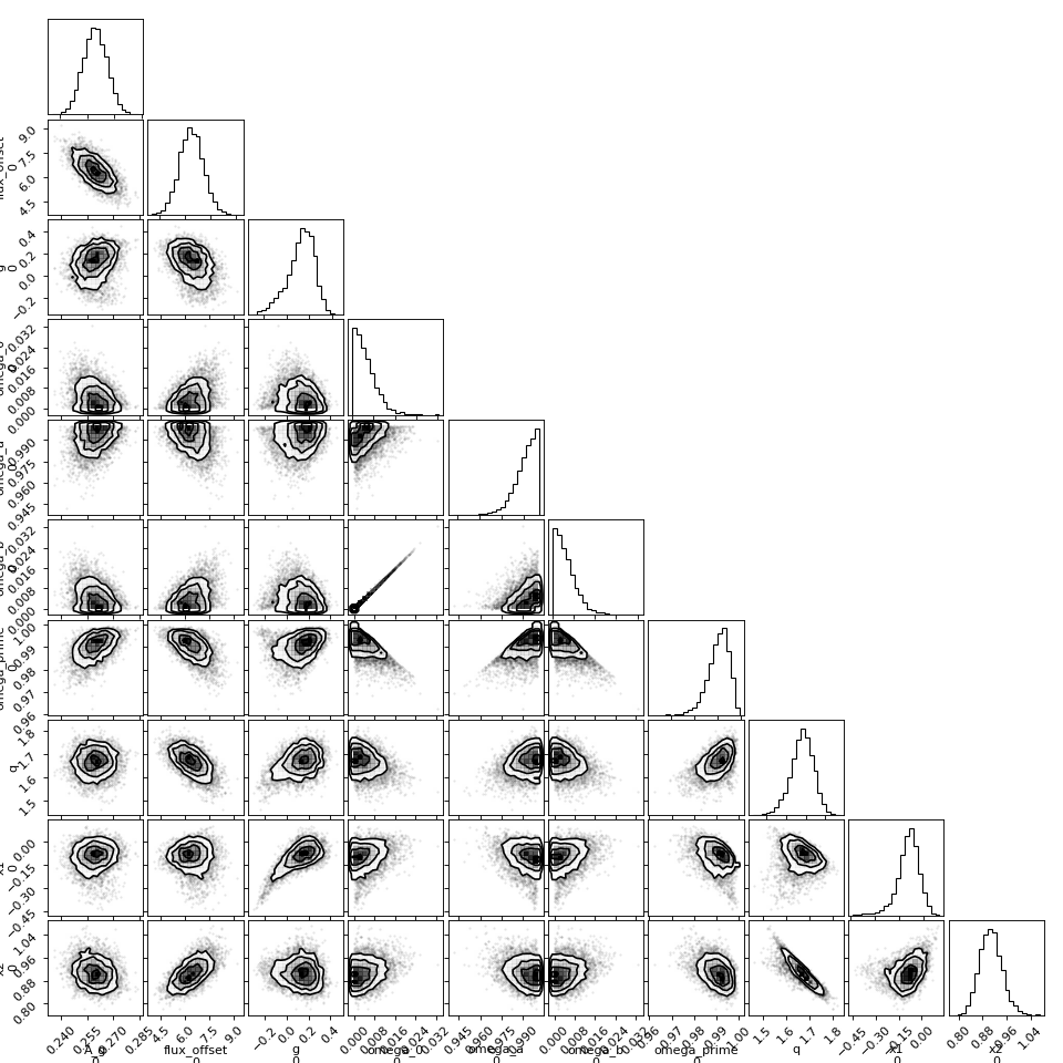
# make a corner plot
corner(
    result,
    quiet=True,
);

# plot several models generated from a few posterior samples:
plt.figure()
plt.errorbar(binphase, binflux, binerror, fmt='o', color='k', ecolor='silver')

n_models_to_plot = 50
keys = ['omega_0', 'omega_prime', 'x1', 'x2', 'A_g', 'flux_offset']

for i in range(n_models_to_plot):
    sample_index = (
        np.random.randint(0, high=mcmc.num_chains),
        np.random.randint(0, high=mcmc.num_samples)
    )
    omega_0, omega_prime, x1, x2, A_g, offset = np.array([
        result.posterior[k][sample_index][0] for k in keys
    ])
    flux_ratio_ppm, g, q = reflected_phase_curve_inhomogeneous(
        binphase, omega_0, omega_prime, x1, x2, A_g, a_rp
    )
    flux_model = flux_ratio_ppm * eclipse_kepler + offset
    plt.plot(binphase, flux_model, alpha=0.1, color='DodgerBlue')
plt.gca().set(
    xlabel='Phase',
    ylabel='$F_p/F_\mathrm{star}$ [ppm]',
    title='Kepler-7 b'
)

(Source code, png, hires.png, pdf)

(png, hires.png, pdf)

The draws from the posteriors for each parameter produce phase curve models that are asymmetric, which match the shape of the observations well.